Rowhammer Lab
Table of Contents
- Part 1: Map Virtual and Physical Addresses (10%)
- Part 2: Observing Bitflips in the Wild (30%)
- Part 3: Find Your Own Aggressor Rows (30%)
- Part 4: Protecting Against Bit-Flips using Error Correcting Codes (30%)
Lab Details
The Rowhammer Lab was released on March 22, and is due on April 13.
Collaboration Policy
Our full Academic Honesty policy can be found on the Course Information page of our website. As a reminder, all 6.S983 labs should be completed individually. You may discuss the lab at a high level with a classmate, but you may not work on code together or share any of your code.
Introduction
In lecture, you learned how a Rowhammer attack works. In practice, however, there are several challenges in practice to pull such an attack off.
First, when we write a C/C++ program, the program uses virtual addresses, which need to be translated to physical addresses before accessing any storage structures, including the DRAM. In addition, physical addresses are distributed into different DRAM banks using a bank mapping function to improve memory parallelism. To conduct successful Rowhammer attacks, we will need to reverse engineer this bank mapping function.
We will guide you through the process of launching real Rowhammer attacks, and explore what we might do to protect against them in this lab. In Part 1, you will examine how virtual to physical address mapping works in Linux. In Part 2, you will be given the physical addresses of a victim row and a few aggressor rows. By implementing a hammer strategy, you will be able to observe bitflips in the wild. In Part 3, you will be only given a victim row, and you need to extend your knowledge of DRAM geometry to find effective aggressor rows to hammer. In Part 4, you will try to implement a software mitigation against Rowhammer attacks.
Getting Started With the Lab Infrastructure
Due to the intrinsic physical requirements of the Rowhammer vulnerability, your experiments must be run on the 6.S983 lab machines. These machines have been verified to reliably exhibit rowhammer characteristics, and your answers to some questions will be specific to their architecture/DRAM configuration. There are fewer machines than students, so machines will be time shared using HTCondor. You will use arch-sec-1.csail.mit.edu to develop and build your code, and use HTCondor to remotely launch your attack code on one of the vulnerable machines (csg-exp[6-10].csail.mit.edu).
You should not access these vulnerable machines (
csg-exp[6-10]) directly, as you may interfere with another student’s experiments. A vast majority of this lab also requires your code to be run under elevated privileges, which is handled automatically (and only possible) while running your code under HTCondor.
Configuration
Your assigned machine information has been emailed to you. Before starting the lab, edit
launch.condorand update theRequirementsline to match the specific machine assigned to you. Make sure not to include the.csail.mit.edusuffix.
Using HTCondor
You cannot directly run your attack code on the vulnerable machines using ./attack_code. You will use HTCondor to launch your attack code using a bash script prepared by us and use the following commands to interact with HTCondor.
bash launch.sh [BINARY FILE]: run the specified binary file in your assigned remote machine. The output will be placed in[BINARY FILE].out, and any errors generated by your code will be placed in[BINARY FILE].error.condor_q: Check the status of your job, including its place in the queue. This command also prints the id of your job. If your job is held, you can see more debugging information by issuing thecondor_q -holdcommand.condor_rm [ID]: Kill your job specified by the id. Note that Condor will kill your job after 5 minutes of execution, to allow other students to use the machine.cat [BINARY FILE].out: Check the output of your job by opening the corresponding output file. Feel free to use any other editor commands.cat [BINARY FILE].error: Print all the errors experienced by your job by opening the corresponding error file. Again, feel free to use any other editor commands.
Here is an example of using HTCondor to run a program which prints Hello World.
$ make

$ bash launch.sh part0
  Submitting job(s).
  1 job(s) submitted to cluster XX.
  All jobs done.

$ condor_q
  -- Schedd: arch-sec-1.csail.mit.edu : <127.0.0.1:9618?... @ 01/27/22 13:45:13
  OWNER    BATCH_NAME    SUBMITTED   DONE   RUN    IDLE  TOTAL JOB_IDS
  pwd      ID: 56       1/27 13:45      _      _      1      1 56.0

$ cat part0.out
  Hello World!
Before continuing, run the Condor commands as above, and ensure that you can interact with your assigned machine correctly. Reach out to the course staff if things do not work as expected.
Part 1: Map Virtual and Physical Addresses (10%)
DRAM uses physical addresses while programs we actually run (including our C/C++ code) uses virtual addresses. In this part you will bridge the gap between these two address spaces. Specifically, you will implement two functions: one translates a virtual address to its corresponding physical address, and the other works in an opposite direction by conerting a physical address to its virtual address. The code you developed here will be reused in the subsequent parts of this lab.
Code Skeleton
The source code (that you will modify) can be found in src/, and is separated into folders corresponding to different parts of the lab.
src/params.hh: Defines several key parameters, including the size of a hugepage (e.g. 2MB), the size of a DRAM row, etc.src/verif.hh: Contains declarations for functions which will help you check your solutions, and will be used for grading.src/shared.hhandsrc/shared.cc: Contains functions which are used across the whole lab - in each part of the lab you will be asked to complete a subset of the included functions.
You can compile the code by running the command make at the root of the repository, which will create five executable files (part[0-4]) in the bin/ folder. Note that you will need to re-run make each time you change your code to re-compile it. For example, you can run the following commands and observe whether you see the following output.
$ make

$ ./bin/part1
    ERROR: Root permissions required!

$ bash launch.sh part1
    Submitting job(s).
    1 job(s) submitted to cluster XX.
    All jobs done.

$ cat part1.out
    Part 1 Test FAILED: Incorrect number of pages in PPN_VPN map (current number of entries: 0)
Before continuing, run
makeand make sure the code compiles successfully (the provided output should match!)
Linux’s pagemap interface
The machines in this lab used paged virtual memory. If you need a reresher on this topic, check out 6.1910’s lecture slides on virtual memory. Linux conveniently provides the pagemap interface that allows userspace programs to examine page tables and related information. For a running process, its pagemap interface can be accessed via the file /proc/self/pagemap.
Here we explain the internal organization of the /proc/self/pagemap file in order to assist you in understanding the skeleton code in shared.cc. The pagemap file is a binary-encoded file containing a sequence of 64-bit values where each value corresponds to a virtual page (assuming a page size of 4KB). The N-th 64-bit value corresponds to the N-th virtual page. The figure below indicates the semantics for each page entry.
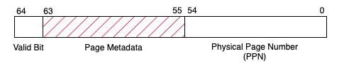
Example Page Map Entry
Bits 0-54 of the entry is the physical page number (PPN), if the page is present in memory. Bit 63 indicates whether the page presents in memory or not. The remaining bits have their own meaning, which are not relevant for this lab. The complete information can be found in the corresponding Linux kernel documentation page.
In the virt_to_phys function in shared.cc, you will translate a given virtual address to its corresponding physical address. At a high-level, the virt_to_phys function will do the following:
- Given a virtual address, derive the address’ virtual page number (VPN).
- (provided) Read
pagemapto find the corresponding page table entry. - (provided) Extract the physical page number (PPN) from the page table entry.
- Compute the physical address from the physical page number (PPN).
1-1 Exercise
Complete the
virt_to_physfunction insrc/shared.cc. Your implementation should derive the virtual page number from a given virtual address, and compute the corresponding physical address from the physical page number returned frompagemap.
Translating in the Other Direction
You also need to implement a function to translate a given physical address back to its virtual address. To do this, you will populate the PPN_VPN_map data structure in shared.cc. PPN_VPN_map is a dictionary implemented using C++’s std::map syntax, with physical page numbers as keys and virtual page numbers as values. For more information related to C++ and examples of how to use the std::map object, refer to the recitation materials.
Note that, the PPN_VPN map assumes 2MB pages as opposed to the 4KB page used by the pagemap interface. Throughout this lab we will exclusively use 2MB hugepages, as they simplify the manipulation of the physical bits relevant to DRAM addressing. In the later parts of this lab, we allocate a large 2GB block of hugepage-backed memory, which will be later used for hammering addresses. In setup_PPN_VPN_map (in shared.cc), you will need to populate the PPN_VPN_map with the corresponding (PPN,VPN) pairs for each 2MB page in the 2GB region.
One quirk with C++ maps is that C++ will return 0 (i.e.
NULL) instead of throwing an error if you try to retrieve a value which isn’t in the map. You will not encounter any non-zero virtual page numbers in this lab, so you may want to check for lookups which return zero!
1-2 Discussion Question
In a 64-bit system using 4KB pages, which bits are used to represent the page offset, and which are used to represent the page number? How about for a 64-bit system using 2MB pages? In a 2GB buffer, how many 2MB hugepages are there?
1-3 Exercise
Complete the
setup_PPN_VPN_mapfunction and thephys_to_virtfunction inshared.cc.
The output of part1 (launched on Condor using bash launch.sh part1) will tell you whether your PPN to VPN map was correctly constructed.
Submission and Grading
You will need to submit shared.cc to your assigned Github repository. You should not modify other files. This part is autograded.
Part 2: Observing Bitflips in the Wild (30%)
Now that you have the virtual and physical address translation under control, you will be able to implement a basic Rowhammer attack and observe bitflips on a real machine. You will implement the double-sided rowhammer attack, report the probability of observing bit flips, and evaluate how the choices of addresses affect the effectiveness of the attack.
We’ve pre-profiled the lab machines for rows vulnerable to rowhammer and provided you with the physical addresses of victim rows and potential aggressor rows below. Note that, these addresses are all physical addresses. You will use these physical addresses to activate the rows in question.
| Machine | Victim | Row Above (A) | Row Below (B) | Distant Row (C) | Same Row ID, Diff. Bank (D) |
|---|---|---|---|---|---|
| csg-exp6.csail.mit.edu | 0x753C1000 | 0x753E3000 | 0x753A7000 | 0x75349000 | 0x753C3000 |
| csg-exp7.csail.mit.edu | 0x75381000 | 0x753A3000 | 0x7536F000 | 0x75309000 | 0x75383000 |
| csg-exp9.csail.mit.edu | 0x75380000 | 0x7536E000 | 0x753A2000 | 0x74380000 | 0x75382000 |
| csg-exp10.csail.mit.edu | 0x7B560000 | 0x7b58e000 | 0x7b542000 | 0x7A560000 | 0x7B562000 |
Attack Outline
In the main function (in part2.cc), we have provided code to collect statistics and report the observed bitflips. You should not modify the file part2.cc. Your task is to implement your hammer strategy inside the hammer_addresses function (in hammertime.cc). We provide a description of the high-level attack flow and some hints below:
-
Prime the victim row to set its content to a known value (for example, all ones), which will be used for comparison in Step 3. For our specific DRAM configuration, a row is of size 2^13 = 8KB.
-
Hammer two rows, repeatedly alternatively accessing two attack rows DRAM 5 million times.
-
Probe the victim row, compare the read results with the primed values, and check whether any bit has been flipped.
- When priming rows, ensure that you’re priming the entire row, and priming to row boundaries correctly.
- When hammering rows, not that, after an address is accessed, it will be fetched into the cache. Subsequent accesses will become cache hits. You will need to come up with a plan to ensure your accesses to the two addresses always miss the cache and access the rows in DRAM.
- To access a row, you only need to access one address belonging to that row.
- When you are writing your code, you may need to convert between integers (
uint64_t) and pointers (uint8_t *) and vice-versa. You may find C++’sreinterpret_castuseful in performing these conversions:uint64_t addr = 0xDEADBEEF; // A 64bit integer // Cast the 64bit integer to a pointer volatile uint8_t * addr_ptr = reinterpret_cast<volatile uint8_t *>(addr); uint8_t tmp = *addr_ptr; // Read using the casted pointer
2-1 Exercise
Fill in the victim address (
addr_victim) and addresses A-D (addr_[A-D]) inpart2.hhusing the addresses for your assigned machine. Then, complete thehammer_addressesfunction.The
part2.cccode will use your function to hammer each aggressor pair 100x, and report how often the attack succeeds (i.e. observes at least one bit flip). Report your results in a table like below. You should (at least) see some bitflips using pair A/B (i.e. double-sided rowhammering).
Hammering Pairs A/B A/C A/D Number of Successes (100 trials)
2-2 Discussion Question
Do your results match your expectations? Why might some attacker pairings result in more flips than others? Do you expect any of the pairs to never cause a flip?
Submission and Grading
This part is graded manually based on the following submitted materials: code and pdf file.
-
Code: You will need to submit
part2/hammertime.ccto your assigned Github repository. You should not modify other files. -
Discussion Questions + Exercises: A pdf with your solutions, uploaded to gradescope.
Part 3: Find Your Own Aggressor Rows (30%)
In Part 2, we provided you with physical addresses to hammer and told you which rows are adjacent to the victim row. You may have noticed that adjacent rows are not always consecutive in physical memory, such as the victim address (“Address A”) and “Address B”. This is because DRAM is physically organized into DIMMs, Channels, Ranks, and Banks, necessitating its own addressing scheme. You can refer to the detailed address mapping of DRAM in the lecture slides. In our lab machines, there are 16 banks, making the bank ID a 4-bit binary value. Each of the four bits of the bank ID is computed by XORing a selection of bits from the physical address, as shown in the figure below.
Specifically, the each bit in the bank ID is computed by XORing some of the “Bank XOR Bits” (bits 13-16) with some bits in the row ID (bits 20-17). The bits involved in this derivation are shown in the figure below.
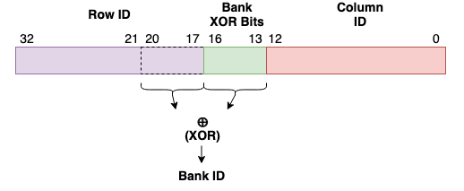
Physical address bits involved in bank ID generation
The exact XOR functions used are proprietary, and we don’t provide them to you in this lab!
In this part, you will be provided the physical addresses of a few victim rows. You will need to come up with a plan to locate the rows adjacent to these victims (within the same bank) in order to trigger vulnerble bitflips as you did in Part 2.
You will first implement a strategy to detect DRAM bank conflicts, which will allow you to determine whether a given pair of addresses map to the same DRAM bank or not. After that, you will have some freedom to decide how to use this information to find aggressor rows. You’re welcome to come up with your own strategy, or employ our suggested methods.
Detecting Bank Collisions via Side Channels
If two addresses are mapped to the same bank, when accessed, there will be bank collisions which result in longer observable access latencies. Therefore, bank collisions can be detected via timing side channel attacks, which you should be very familiar with from previous labs. This time, however, instead of attacking the caches you can exploit either memory bus contention, row buffer contention, or both. Here are two possible timing strategies you might consider employing:
-
Detecting Row Buffer Conflicts: Given two physical addresses x and y, make sure both of the addresses are not cached. First, access address x from DRAM (filling the row buffer with x’s row). Next, access address y from DRAM, which will close the row buffer opened by x if it maps to the same bank. Finally, access address x again from DRAM and measure its access latency (making sure it was flushed from the cache beforehand). If x and y are mapped to the same bank but different rows, then this access will result in a row buffer miss and should take a longer time to complete.
-
Detect bus contention and row buffer conflicts: Given two physical addresses x and y, again make sure both of the addresses are not cached. Access the two addresses back-to-back without memory fences in between and measure their collective access latency. If the two addresses are mapped to the same bank and different rows, they will cause memory bus contention in addition to row buffer conflicts, and thus will result in even longer latency.
Implement the approach of your choice in measure_bank_latency (in the file shared.cc). The function takes two virtual addresses as arguments and measure the access latency using one of the above approaches. We have provided two reference implementations and python scripts for you to check whether your code works correctly or not.
Code skeleton
You do not need to modify any of these files!
src/part3/part3_1.cc: This file contains the main function which callsmeasure_bank_latency, populates two arrayssame_bank_latencyanddiff_bank_latency, and outputs latency results that can be processed by the python scripts.bin/part3_reference1: A reference implementation that detects only row buffer conflicts.bin/part3_reference2: A reference implementation that detects both bus contention and row buffer conflicts.src/part3/run.py: Similar to Lab 1, it launches a target binary program 100 times to collect statistics in a folderdata. The folderdatawill be overwritten each time you run the script.src/part3/graph.py: Similar to Lab 1, it takes the statistics in folderdataand generate a histogram in the foldergraph.
Once you’ve completed your implementation of measure_bank_latency, collect and generate the timing histogram by running bash launch.sh part3_1. The final timing histogram will be written to the graphs/ folder. To view the histogram, either copy it to your own machine via SCP, or run gv graphs/graph_name.pdf to view the histogram over the network.
If you are viewing the histogram over the network, you may need to set up x-forwarding/add the forwarding flag when connecting via ssh, i.e.
ssh arch-sec-1.csail.mit.edu -X).
3-1 Exercise
Complete the function
measure_bank_latency, and use the provided python scripts to generate a histogram. You can use the reference implementations to see whether your code works correctly or not.
3-2 Discussion Question
According to the histogram, what is the appropriate threshold to determine whether two addresses are mapped to the same bank or not?
Locating Aggressor Rows
We have emailed you the physical addresses of 3 potential victim addresses (at least one of which we have verified to be vulnerable). You are asked to find effective aggressor addresses to verify whether each of these victims are vulnerable or not. You will use some heuristics to do the following:
- Construct a set of aggressor row candidates, consisting of all addresses with adjacent row IDs. In other words, if we’re examining a victim address with row ID N, construct the set of addresses with row ID N-1 and N+1, with identical column ID values.
- From this set of candidates, determine the two rows which map to the same bank using the side channel that you have developed, and
- Use the derived aggressor rows to perform rowhammer and see whether a bitflip can be triggered.
3-3 Exercise
List the set of addresses which have adjacent row IDs (column 2). For each of these addresses, test whether or not they fall into the same bank (column 3) as the victim address. Finally, validate whether these addresses can be used to trigger a bit flip in the victim (column 4).
Victim Address Addresses with Adjacent Row IDs Pair of Tested Addresses that Fall in the Same Bank Rowhammer Triggered? Email Provided A Email Provided B Email Provided C
Submission and Grading
This part is graded manually based on the following submitted materials: code and a pdf file.
-
Code: You will need to submit file
part3/shared.ccandpart3/part3_2.ccto your assigned Github repository. You should not modify other files. -
Solutions: You will include the generated histogram in the pdf file with the answers to the discussion questions.
Part 4: Protecting Against Bit-Flips using Error Correcting Codes (30%)
Now that we have demonstrated bit-flips in the wild, let’s now explore a potential defense to Rowhammer: Error Correcting Codes (ECC). Error correcting codes are encoding schemes which add redundancy to stored data, allowing for the recovery of said data even if some bits are flipped. To do so, ECC takes in the data to be protected, and generates additional parity bits which help detect and correct errors.
Types of ECC
There exists many different flavours of ECC, each with their own benefits and drawbacks.
-
Repetition Codes: The simplest code is the repetition code, which duplicates each bit in the data multiple times. For example, if we want to protect a stored value
1011in memory, we can replicate it in memory some number of times In this case, a 3-repetition code would store1011 1011 1011). -
Single Parity Bit: If we’re concerned about storage overhead, we can detect errors by calculating the parity of the data by XORing the data bits together. For example, the parity bit for
1011is1, and the parity bit for1001is0. Observe that a single bit flip in the data results in the parity bit changing! -
Hamming Codes: Hamming codes use multiple parity bits to deal with bit errors. There exists many variants of the Hamming encoding scheme, with the most common one being Hamming(7,4), i.e. 4 data bits protected by 3 parity bits.
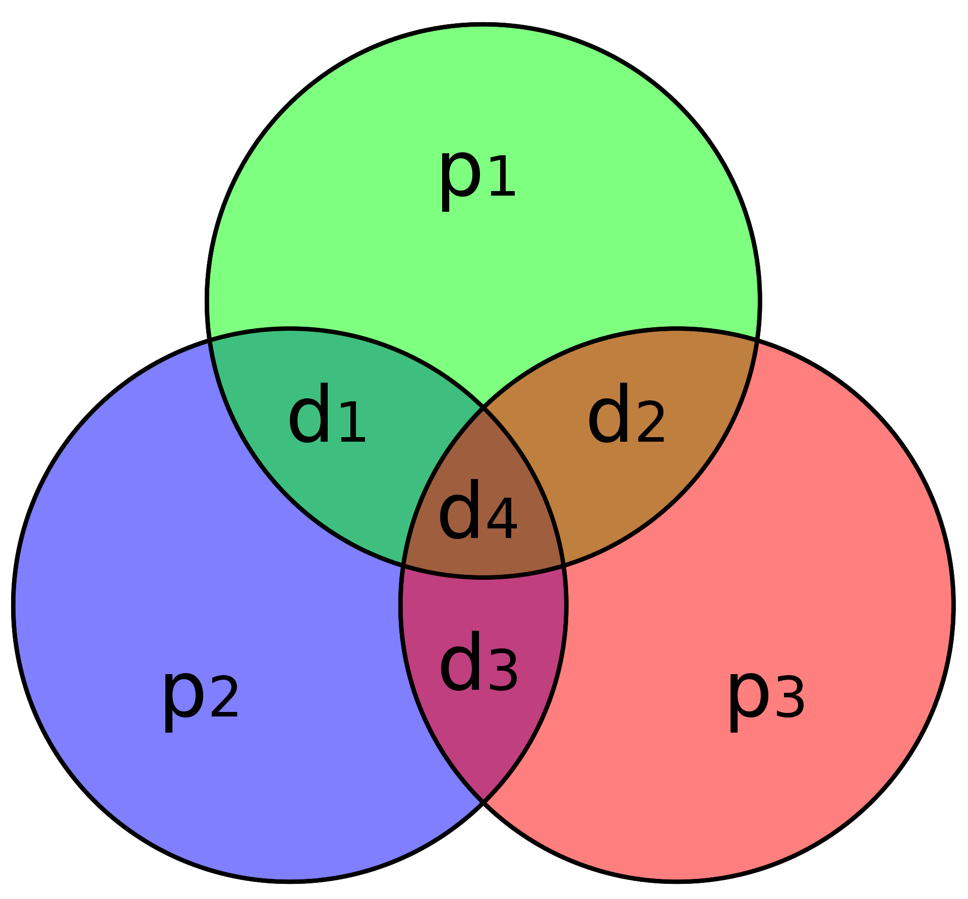
(7,4) Hamming Code Example (Source)
A graphical depiction of the parity encoding for the 4 data bits (d1 to d4) is shown in the above figure. Rather storing information about all bits at once, the first parity bit p1 only considers the parity of data bits 1, 2, and 4, and is calculated by XORing d1,2,4 together. After calculating the parity bit, note that the XOR of d1,2,4 and p1 will be zero (thus, in the figure, the XOR of all elements in the circle should always be zero). Thus, if any single bit in a circle gets flipped, the parity of the circle also flips (indicating an error).
By using parity bits in an overlapping fashion, the Hamming(7,4) code can detect one or two bit flips, and can correct a single bit flip. This error correction capability is commonly referred to as SECDED (Single Error Correction Double Error Detection).
#/media/File:Hamming(7,4).svg)
4-1 Discussion Question
Given the ECC type descriptions listed above, fill in the following table (assuming a data length of 4). For correction/detection, only answer “Yes” if it can always correct/detect. We’ve filled in the first line for you.
ECC Type Code Rate
(Data Bits / Total Bits)Single Error Detection?
(Y/N)Single Error Corrrection?
(Y/N)Double Error Detection?
(Y/N)Double Error Correction?
(Y/N)Triple Error Detection?
(Y/N)1-Repetition (No ECC) 1.0 N N N N N 2-Repetition 3-Repetition Single Parity Bit Hamming(7,4)
Implementing ECC in Hardware
Hamming coded ECC is frequently found in datacenter DRAM, primarily defending against soft errors. In this section we’ll complete a software implementation a Hamming(22,16) encoding scheme, which is used in real hardware.
4-2 Discussion Question
What is the code rate of Hamming(22,16)? Compare the space requirements for storing equal amounts of data using both Hamming(22,16) and Hamming(7,4).
4-3 Discussion Question
Fully read the description of Hamming(22,16). When a single bit flip is detected, describe how Hamming(22,16) can correct this error.
Now, let’s write some code in part4.cc! For this part, you do not need to use condor (and can run ./bin/part4 directly). You will be responsible for writing three parts of the implementation: computing the parity bits, detecting errors, and correcting them (if possible).
For your convienence, we’ve provided the following helper types/functions in part4.hh:
struct hamming_struct: A C++ struct which contains a data and parity pair.struct hamming_result: Stores an error type (one ofNO_ERROR/SINGLE_ERROR/DOUBLE_ERROR/PARITY_ERROR) and computed syndrome.getBit(data, pos): Returns the value of the bit at positionposwithindata.flipBit(data, pos): Flips the bit at positionposwithindata.isParityBit(bitNum): Returns whether bitNum corresponds to a parity bit in the Hamming(22,16) encoding.extractEncoding(encoded): Takes a 22 bit encoded ECC value, and extracts the parity and data bits (returned in ahamming_struct).embedEncoding(hamming_struct): Takes in ahamming_structand returns the combined ECC value.
First, complete the function (genParity) that calculates the parity bits (P5-P0) for an input piece of data that needs to be protected. The parity equations are shown on page 2 of the Xilinx document. For convenience, we’ve included the parity_eqs array in part4.cc which describes the parity equations in an array representation.
4-4 Exercise
Complete
genParity(). You should see a message telling you that your parity value is correct when you run./bin/part4(make sure to compile your implementation usingmake!).
Now, write a function (findHammingErrors()) that takes in an encoded ECC value and determines whether there is an error. This function should return the error type and the syndrome (both as described in the Xilinx document).
Table 2 in the Xilinx document summarizes the conditions required for a given error type.
Finally, write a function (verifyAndRepair()) which uses the information gained from findHammingErrors() to determine a good course of action. If there is no error, or an unrecoverable error, verifyAndRepair() should return the original value. If there is a single bit error (including parity errors), verifyAndRepair() return the data with the error corrected.
4-5 Exercise
Complete
findHammingErrors()andverifyAndRepair(). You should seeAll tests passed!reported.
4-6 Discussion Question
Can the Hamming(22,16) code we implemented always protect us from rowhammer attacks? If not, describe how a clever attacker could work around this scheme.
Submission and Grading
Your part4.cc will be graded automatically, checked against 5 random inputs. As always, submit your discussion questions within your gradescope pdf.
Acknowledgements
Contributors: Peter Deutsch, Miguel Gomez-Garcia, Mengjia Yan.